Introduction
Our model uses a combination of polling averages and historical voting data (quantified via the BPI) to form election predictions for this year’s cycle. Choosing how to weight the polling averages versus the BPI when taking the average of the two metrics is an important consideration. Relying too heavily on the polls to make our prediction may be problematic if the polls are not representative of the voting population, while overweighting the BPI means that we fail to account for recent changes in public opinion.
Our class decided to vary the weight given to the polling average based on the number of polls available for the race and the recency of those polls. We felt that polling averages are more reliable when they are based on the results of many polls rather than just a few. We also agreed that recent polls are likely more accurate and reflective of voters’ current opinions than older polls. For this reason, we weighted the polling average more heavily for races with a greater number of polls and more recent polls. Our formula for determining the weight of the polls was
where `n_30` is the number of polls in the last thirty days for a certain race and `n` is the total number of polls for that race.
The numerator of the coefficient on the arctan function represents the horizontal asymptote of the curve, or the maximum possible weight of the polls. As the number of polls for a particular race approaches infinity, the weight given to the polling average approaches 95% (1.9 divided by 2). Our initial formula also takes into account the number of polls which were conducted within the past thirty days and gives that number greater weight than the number of polls in total.
These coefficients were chosen by taking a simple average of the results of a class poll. We wondered what our model would look like if we had used different coefficients. Our goal is to determine whether or not tampering with these aspects of our formula will drastically impact the ORACLE’s predictions. In this study, we change the maximum weight of the polls, remove our weighting based on age, and do both together.
Methodology
In order to compare the predicted percentages from the official formula with results from our modified formulas, we used data from October 24th and ran our model an additional five times, one time with each new formula we created. Using the data from these simulations, we ran t-tests on the original model data and each of our new formulas to determine the impact of our new formulas on the original model.
The new formulas and how we will refer to them are listed below:
| Name | Formula | What it changes |
|---|---|---|
| Formula 1 | `w=frac{1.2}{pi}arctan(1.75n_{30}+0.05n)` | Decreases the maximum poll weight to 60% |
| Formula 2 | `w=frac{1.5}{pi}arctan(1.75n_{30}+0.05n)` | Decreases the maximum poll weight to 75% |
| Formula 3 | `w=frac{1.9}{pi}arctan(0.5n)` | Does not consider poll recency in calculating the total weight of polls |
| Formula 4 | `w=frac{1.2}{pi}arctan(0.5n)` | Does not consider poll recency in calculating the total weight of polls and decreases the maximum poll weight to 60% |
| Formula 5 | `w=frac{1.5}{pi}arctan(0.5n)` | Does not consider poll recency in calculating the total weight of polls and decreases the maximum poll weight to 75% |
Results
We obtained our results by using Minitab to run paired t-tests and generate graphs.
Formula 1
Formula 2
Formula 3
Formula 4
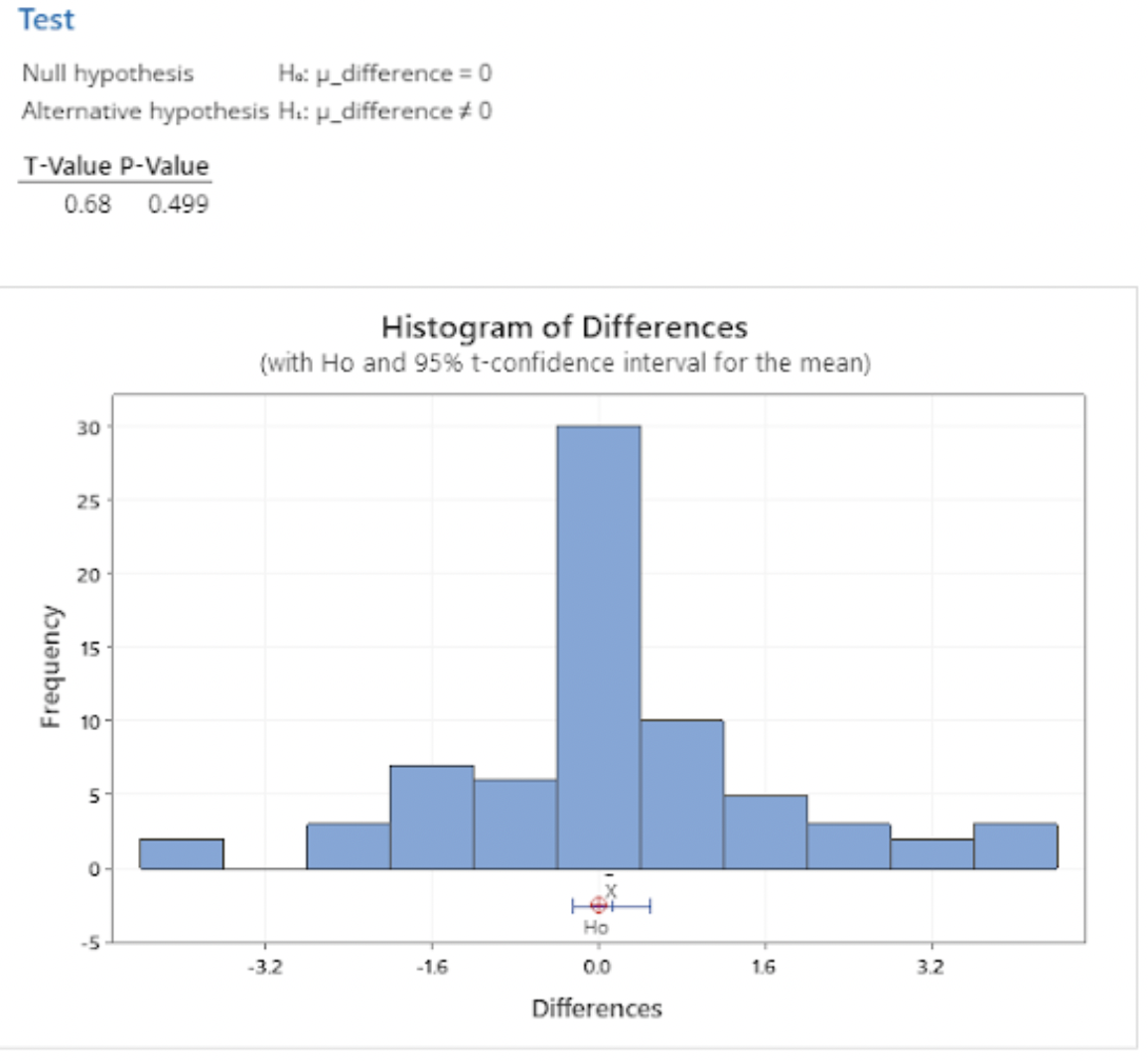
Formula 5
Discussion and Conclusions
Our null hypothesis is that there is no difference between the results of our official formula and each of the modified formulas. Our alternative hypothesis is that there is a difference. We decided to use a significance level of p = 0.05 for this study, where p-values higher than 0.05 indicate that our modified formulas likely do not have a significant effect on the results.
Formula 1: 60% Maximum Poll Weight
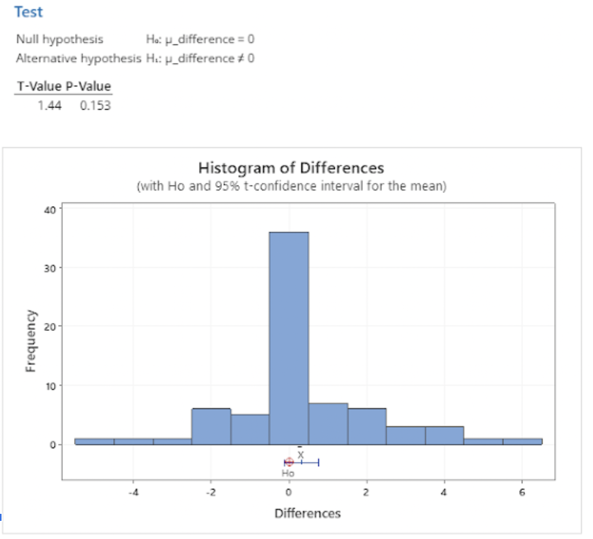
The t-test between the original formula and Formula 1 returned a t-value of 1.44, which equates to a p-value of 0.153 — in other words, if we assume that there is no difference between the prediction using the official equation and ours, there is a 15.3% chance that we would see the differences we observed in the data just based on sampling variance. This effectively means that a maximum poll weight of 60% has little to no effect on the model when compared to a 95% maximum poll weight. While the overall effect of this new formula was negligible, there are some standout races that were impacted more by this formula, including the Alaska Senate race and the Vermont governor race. The Alaska Senate race got closer using this formula, with Republicans expected to win an additional 6.29% of the vote for a total of 46.87%, which is still below that 50% threshold they would need to win. Vermont’s Governor race also closed in, but at the Democrats’ advantage instead; this formula predicted an additional 5.25% for them, ending up with 47.16% of the vote — also not enough to push them into winning territory.
Formula 2: 75% Maximum Poll Weight
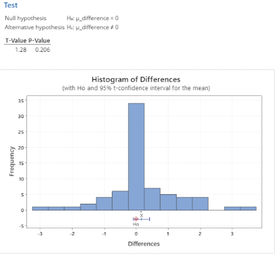
Our t-test between the original formula and Formula 2 returned similar results, with a t-value of 1.28 corresponding to a p-value of 0.206. This is again higher than our significance level, indicating that changing the maximum poll weight to 75% had little effect on our current model. Alaska’s Senate race shifted the most using this formula but only changed by 3.59 percentage points; Democrats remain in the lead despite this change, though.
Formula 3: No Age Weighting
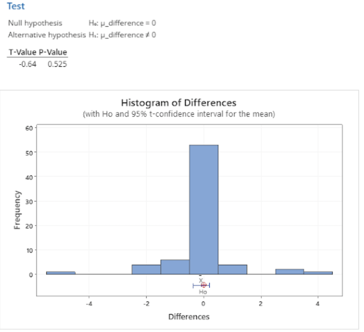
Our results here also suggested that the effect of age weighting in our official formula is minimal: we observed a t-value of -0.64 and a p-value of .525, the greatest of any of our modified formulas, indicating that this formula had the least effect on the predictions that our official model generated. The two races the most affected by this formula were Maryland’s Senate race and the Kansas governor race, the latter being one of the four races that flipped. The flipped races are discussed below. As for Maryland’s Senate race, this formula predicted a 4.15-point increase in Republican votes, bringing them up to 45.05%.
Formula 4: No Age Weighting, 60% Maximum Poll Weight
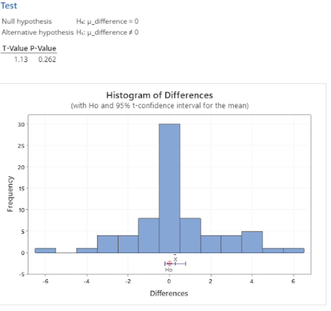
The t-test we performed for this equation gave us a t-value of 1.13 and a corresponding p-value of 0.262, well above our significance level. The races that swung more than 5% in either direction include the Vermont Governor race and Alaska Senate race. Vermont’s Governor race shifted 6.11 percentage points closer to the center, with Republicans still in the lead; Alaska’s Senate race shifted 6.44 percentage points closer to the center, with Democrats remaining in the lead. Other races that shifted fewer than 5 but greater than 4 percentage points include Maryland’s, Nebraska’s, New York’s, and Oklahoma’s Governor races and Louisiana’s Senate race.
Formula 5: No Age Weighting, 75% Maximum Poll Weight
Finally, the t-test we performed to compare our last equation to the original returned a t-value of 0.68, translating to a p-value of 0.499, which is quite a bit greater than our significance level of 0.05. No races shifted more than 5% using this formula.
Race Flips
There are 4 races where our modified equations flip the vote percentage from majority Democrat to majority Republican or vice versa. Polling data is largely responsible for these changes. Any recent gains (within the last 30 days) for a lagging candidate would have been ignored by our formulas that remove weighting based on recency. In addition, polls that heavily favor one candidate in races that have a BABOON close to 50% would have less effect on our prediction with the formulas that lower overall poll weight.
Arizona Senate
The first flipped race is the Arizona senate race between Mark Kelly (D, incumbent) and Blake Masters (R). Our original model forecasted a 51.5% vote share for Kelly on October 24. With the exception of our formula that only removes weighting based on age (formula 3), our other formulas granted Masters a 2 to 4 percentage point bonus, enough to give the seat to the Republican. Changing the weight of the polls makes a difference for this race because Arizona’s BPI and polling averages are very different. The BPI leans heavily Republican, with a historical average democratic vote percentage of only 41.39%. However, in this race, Democratic candidate Mark Kelly is consistently ahead in the polls. By reducing the weight given to the polls, our new formulas allow our model’s Arizona senate prediction to flip Republican, in accordance with the BPI.
Georgia Senate
The Georgia senate race between Raphael Warnock (D, incumbent) and Herschel Walker (R) also flipped when all but one of our new formulas were applied. Once again, the exception was our formula that only removed weighting by poll age. The official model predicted a 50.64% vote share win for Warnock on October 24, but our new formulas added between 1.8 to 3.3 points to the Republican vote share, changing our predicted winner to Walker. Similar to the case of Arizona’s senate race, the flip largely occurs due to the difference between Georgia’s BPI, which strongly favors Republicans, and the polls, which lean slightly democratic.
Wisconsin Senate
Another race that flipped is the Wisconsin Senate race between Mandela Barnes (D) and Ron Johnson (R, incumbent). On October 24, the official model predicted a close win for Johnson, with 50.38% of the vote. Three of our formulas corroborated this prediction, but the other two — the equations which capped the poll weight at 60%, formulas one and four — both predicted a very close win for Barnes instead, with 50.019% of the vote according to formula one and 50.025 according to formula four. For this race, the BPI (50.71%) and polling averages (48.91%) are very close, which means even small changes in the weights used to take the weighted average of the two metrics can result in the state’s flip from blue to red, or vice versa.
Kansas Governor
The final race that flipped was the Kansas Governor race between Laura Kelly (D, incumbent) and Derek Schmidt (R). Our official model’s October 24 prediction gave Schmidt a pretty comfortable win with 55.32% of the vote. However, our third formula, which considered all polls equally instead of giving more weight to recent ones, shifted the prediction just enough to switch sides; if we had used this equation for our official model, we would have estimated 50.18% of the vote for Kelly. Part of the reason for this is that there are only 5 polls available for this race, none of which were taken in the past 30 days. Our time-independent formula gives more weight to the polls than the previous formula did, shifting the overall prediction from Republican to Democrat.
Race Flip Summary
| Race | Original Winner | Original Lean | Formula 1 Lean | Formula 2 Lean | Formula 3 Lean | Formula 4 Lean | Formula 5 Lean |
|---|---|---|---|---|---|---|---|
| Arizona Senate | D | 51.498 | 47.798 | 49.400 | 51.316 (No flip) | 47.657 | 49.225 |
| Georgia Senate | D | 50.645 | 47.449 | 48.819 | 50.553 (No flip) | 47.391 | 48.746 |
| Wisconsin Senate | R | 49.615 | 50.019 | 49.846 (No flip) | 49.625 (No flip) | 50.025 | 49.854 (No flip) |
| Kansas Governor | R | 44.680 | 44.156 (No flip) | 44.381 (No flip) | 50.180 | 47.629 (No flip) | 48.723 (No flip) |
Overall, adjusting the weight given to the polls when combining the polling average with the BPI does not cause significant changes in our model’s predictions. There are only 4 state races where our adjusted formulas cause the predicted win to flip from one party to the other, and these races are generally very tight races with small predicted win margins. Adjusting the weight of the polls has the most significant impact in races where the BPI and the polling average of the state are very different.