Introduction
Our model predicts the percentages for each race by taking a weighted average of two separate estimates, BABOON and the polling averages. On the other hand, the variance in our estimates is calculated by adding extra sources of variance to the sampling variance of polls. We then use these to create a distribution of possible results for the elections, and from these distributions we calculate the probability of a Democrat or Republican majority in the Senate. Clearly, extra sources of variance must be scaled to adjust for their relative importance, so that our estimated probability can be more accurate.
We contend that these scaling constants must be chosen very precisely, and that small changes to the constants can massively affect the simulation results. Because not every possible source of extra variance has been considered by our model, it should be the case that the model underpredicts the true variance. However, an estimated variance near the true variance can still be obtained by adjusting the scaling constants on the considered sources of variance. We believe this method of obtaining variance to be a major flaw in the model because there is no longer any measure of the true variance. This is because it is possible to simply adjust the scaling constants so that the estimated variance is any arbitrary value regardless of the true variance.
Methodology
The ORACLE model incorporates the following two variables into our estimate of polling variance (go to https://polistat.mbhs.edu/methodology for more in depth explanations).

They are then added to polling variance to determine our approximation of variance as follows:

N_30 and n denote the number of polls in a state’s race in the last 30 days and the total number of polls in a state’s race, respectively.
The constants 2 (from VIBE, referred to hereafter as the “A coefficient” or “A”) and 0.08 (GOOFI, referred to hereafter as the “B coefficient” or “B”) were chosen by averaging the proposed values from our team. To investigate the impact of changing these variables, we reran the ORACLE calculation of Democratic win % in the Senate 1,000 times using uniformly and randomly chosen values of A (between 0.5 and 4) and B (between 0.01 and 0.1).
Results
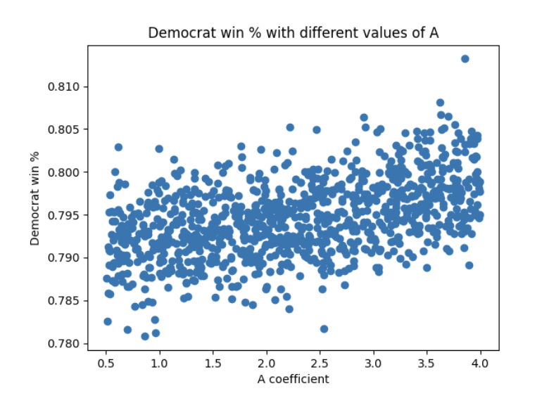
 Figure 1
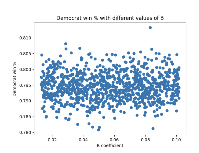
 Figure 2
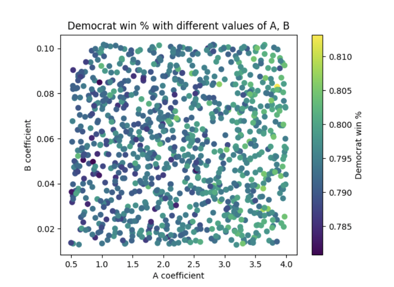
 Figure 3
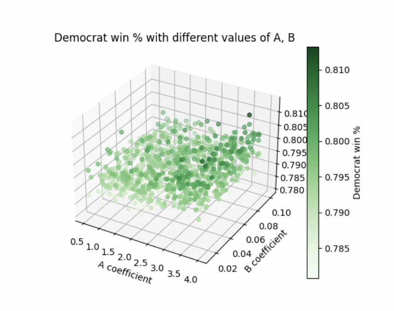
 Figure 4
All simulations captured in Figure 1 assume that the B coefficient is constant at 0.08. Likewise, all simulations captured in Figure 2 assume that the A coefficient is 2. Figure 3 includes simulations that randomly and uniformly pick values for both the A coefficient and the B coefficient. In a sense, it is a combination of the factors visible in Figure 1 and Figure 2. Figure 4 is a different visualization of figure 3. Looks pretty cool, right? :)
Analysis
Figure 1 shows a positive linear relationship between the Democratic win % and the A coefficient. Recall that VIBE, the calculation of which includes the A coefficient, describes additional variance added based on the population of voters or likely voters polled that report being undecided. Different states have significantly different populations of undecided voters. For example, a September poll by Goucher College, covering the Senate race in our home State of Maryland, categorized 11% of respondees as undecided. On the other hand, an October poll by Public Policy Polling, covering the Senate race in Louisiana, categorized 31% of respondees as undecided. Figure 1 implies that giving greater consideration to these undecided voters in individual Senate elections favors the Democrats’ chances of winning a majority in the Senate overall. It appears that states with relatively high populations of undecided voters tend to lean Republican.
On the other hand, Figure 2 shows a lack of correlation between the Democratic win % and the B coefficient. Recall that GOOFI, the calculation of which includes the B coefficient, describes additional variance added based on the state-specific prediction error in previous iterations of the Blair ORACLE. Essentially, it helps us learn from our past mistakes (or at least make an effort to give those mistakes a nod in our model). Figure 2 implies that giving greater consideration to the size of the error in our past predictions favors neither party. It appears that the size of the errors in our previous state-specific predictions is relatively constant between both red and blue states, and that our choice of B coefficient has little impact on our model.
If we consider the specific state of Illinois, the default values for A and B give us a Democratic win percentage of 86.68% but letting A, and B vary can have that number as high as 96.26% or as low as 71.76%, with higher percents when A, B are low and lower percents when A, B are high, as shown in Table 1 below.
| A | B | Dem win % |
|---|---|---|
| 2.0000 | 0.0800 | 0.8668 |
| 1.8254 | 0.1244 | 0.7601 |
| 1.2076 | 0.1175 | 0.7714 |
| 2.9333 | 0.1561 | 0.7176 |
| 3.4436 | 0.1076 | 0.7890 |
| 2.6039 | 0.1244 | 0.7601 |
| 3.3526 | 0.1269 | 0.7562 |
| 1.3649 | 0.1321 | 0.7484 |
| 3.2955 | 0.0728 | 0.8687 |
| 2.5072 | 0.1467 | 0.7288 |
| 2.2922 | 0.0402 | 0.9626 |
| 3.2218 | 0.0702 | 0.8759 |
| 1.1096 | 0.0741 | 0.8654 |
| 3.1316 | 0.0742 | 0.8650 |
| 1.1535 | 0.1407 | 0.7365 |
| 0.9104 | 0.1079 | 0.7885 |
| 1.5025 | 0.1155 | 0.7749 |
| 1.7386 | 0.0959 | 0.8126 |
| 1.3435 | 0.1215 | 0.7648 |
| 2.7532 | 0.0679 | 0.8823 |
| 1.3430 | 0.1336 | 0.7463 |
Table 1: Democratic win percentages for various values of A and B in the Illinois Senate.
Conclusion
It seems that we must carefully consider how much importance to assign to the predictive influence of undecided voters. On the other hand, our overall methodology, which modifies each of the variances of our predictions for each state race based on only the magnitude of the error of previous iterations of the ORACLE, seems to be largely unaffected by our predictive track record. It’s notable that our historical tendency to overpredict in the favor of the Democrats is not compensated for by the construction of our current model.
So, undecided voters are important. But, how important? Compared to an A coefficient of 0.5, choosing an A coefficient of 4.0 gave Dems an additional 0.65% probability of winning a majority. Our hypothesis can be rejected.
While our methodology of choosing these two constants in variance calculation seems to not manifest into a major flaw in our model for the whole nation, for individual states there are large differences.